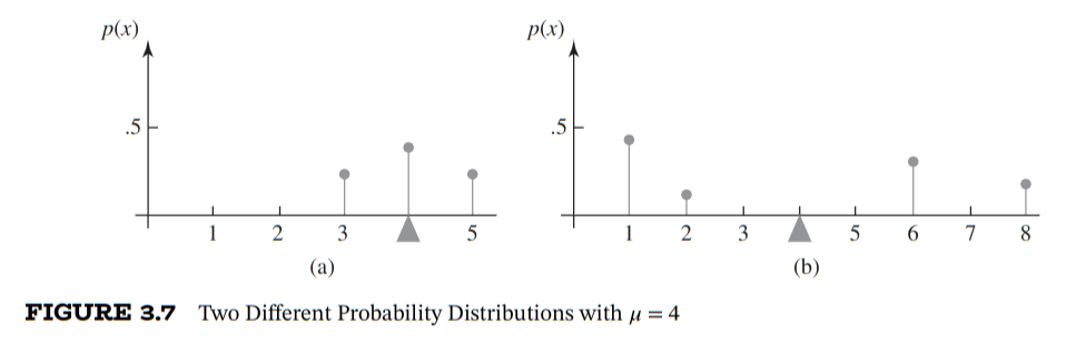
Variance and Standard Deviation of X

Sometimes even though the Expected Value of some distribution equals, they are more/less variant:

Pasted image 20241003164949.png

Although both distributions in the figure above have the same expected value, they clearly are different distributions, where the second is more varied than the first. We have a quantitative way to describe this variance:

Variance, standard deviation

Let $X$ have pmf $p (x)$ and expected value $μ$ . Then the variance of $X$ , denoted by $Var (X)$ or $σ_{X}^{2}$ or $σ^{2}$ is:

Var (X) = \sum_{x \in D} [(x - μ)^{2} p (x)] = E [(X - μ)^{2}]

The standard deviation of $X$ denoted $SD (X)$ or $σ_{X}$ or $σ$ is just:

σ_{X} = \sqrt{Var (X)}

Where does this come from

The idea is that $σ$ is the average distance from $μ$ . Think of the $σ^{2}$ function as doing the norm, so then square rooting will find the distance from $μ$ .

See [[handout05-DiscreteRVs-350F24_annotated.pdf#page=4]] for some examples of computing these.

Chebyshev's Inequality

Let $X$ be a discrete rv with Expected Value $μ$ and standard deviation $σ$ . Then for any $k \geq 1$ :

P (| X - μ | \geq k σ) \leq 1 / k^{2}

That is, the probability $X$ is at least $k$ standard deviations away from the mean $μ$ is at most $1 / k^{2}$ .

Proof
Let $A$ denote the event $| X - μ | \geq k σ$ . Begin by rewriting out the definition of $Var (X)$ :

\begin{aligned} Var (X) & = \sum_{D} [(x - μ)^{2} p (x)] \\ = \sum_{A} [(x - μ)^{2} p (x)] + \sum_{A^{'}} [(x - μ)^{2} p (x)] \\ \geq \sum_{A} [(x - μ)^{2} p (x)] & the other sum \geq 0 \\ \geq \sum_{A} [(k σ)^{2} p (x)] & (x - μ)^{2} \geq (k σ)^{2} \\ = (k σ)^{2} \sum_{A} p (x) \\ = (k σ)^{2} P (A) \\ = k^{2} σ^{2} P (| X - μ | \geq k σ) \end{aligned}

Solving $Var (X) = σ^{2}$ and simplifying gives the desired result. The middle step uses the variance shortcut.
☐

Variance Shortcut

$Var (X) = σ^{2} = E (X^{2}) - μ^{2}$

Proof
See [[handout05-DiscreteRVs-350F24_annotated.pdf#page=5]].
☐
If $h (X)$ is a linear function, then we get the following:

Linear

h

implies linear transformation of

Var, μ, σ

If $h (X) = Y$ is a linear function, then:

Var (a X + b) = σ_{a X + b}^{2} = a^{2} \cdot σ_{X}^{2}

σ_{a X + b} = | a | \cdot σ_{X}