Ch 11 - 13, 15, 19

11.11

Question

Pasted image 20241107171508.png
For context the pdf is:
Pasted image 20241107171727.png

Proof

\begin{aligned} E (X (t)) & = E [\cos (2 π f_{0} t + \frac{π}{4} + \frac{K π}{2})] \\ = \sum_{\forall k} \cos (2 π f_{0} t + \frac{π}{4} + \frac{k π}{2}) \cdot p (k) \\ = \sum_{k = 0}^{3} \cos (2 π f_{0} t + \frac{π}{4} + \frac{k π}{2}) \cdot \frac{1}{4} \\ = \frac{1}{4} [\cos (β (t) + \frac{π}{4}) + \cos (β (t) + \frac{3 π}{4}) + \cos (β (t) + \frac{5 π}{4}) + \cos (β (t) + \frac{7 π}{4})] \\ = \frac{1}{4} \cdot 0 \\ = 0 \end{aligned}

(Here we contract $2 π f_{0} t = β (t)$ ). The last step we notice that $\cos (β + \frac{π}{4}) = - \cos (β + \frac{5 π}{4})$ geometrically (they are always on opposite sides of the unit circle) and similar with the other two terms. They cancel giving a total sum of 0.

\begin{aligned} Var (X (t)) & = E [(X (t) - μ_{X (t)})^{2}] \\ = \sum_{k = 0}^{3} {(\cos (2 π f_{0} t + \frac{π}{4} + \frac{k π}{2}) - 0)}^{2} \cdot \frac{1}{4} \\ = \frac{1}{4} \sum_{k = 0}^{3} \cos^{2} (2 π f_{0} t + \frac{π}{4} + \frac{k π}{2}) \\ = \frac{1}{4} (\cos^{2} (2 π f_{0} t + \frac{π}{4}) + \cos^{2} (2 π f_{0} t + \frac{3 π}{4}) + \cos^{2} (2 π f_{0} t + \frac{5 π}{4} + \dots)) \end{aligned}

Here if we let $a^{2} (t) = \cos^{2} (2 π f_{0} t + \frac{π}{4}) = \cos^{2} (2 π f_{0} t + \frac{5 π}{4})$ and $b^{2} (t) = the other one$ . Then:

Var (X (t)) = \frac{1}{4} (2 a^{2} (t) + 2 b^{2} (t)) = \frac{a^{2} (t) + b^{2} (t)}{2}

Which is:

\begin{aligned} = \frac{1}{2} \cdot (\cos^{2} (2 π f_{0} t + \frac{π}{4}) + \cos^{2} (2 π f_{0} t + \frac{3 π}{4})) \\ = \frac{1}{2} \cdot (\cos^{2} (2 π f_{0} t + \frac{π}{4}) + \sin^{2} (2 π f_{0} t + \frac{π}{4})) \\ = \frac{1}{2} \end{aligned}

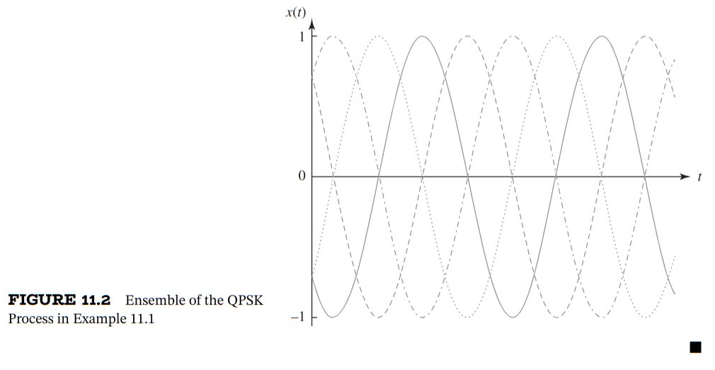
Looking at our figure.

Pasted image 20241107174212.png

Notice that:

The average distribution is centered at $μ_{X} = 0$ , validating that answer.
It's odd that the variance is $\frac{1}{2}$ , implying that $σ_{X} (t) = \frac{\sqrt{2}}{2}$ . It seemed that $σ_{X}$ should be changing over time with the graph, but I guess this makes sense since each point in the graph has the opposite distribution on the other end of the $x = 0$ line.

☐

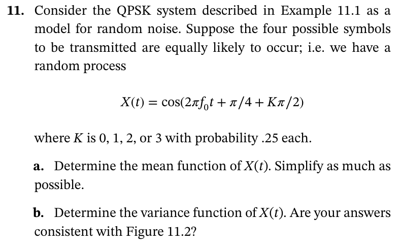
11.13

Question

Pasted image 20241107174527.png

Proof

\begin{aligned} C_{X X} (t, s) & = Cov (X (t), X (s)) \\ = Cov (v_{0} + A \cos (ω_{0} t + θ_{0}), v_{0} + A \cos (ω_{0} s + θ_{0})) \\ = \cos (ω_{0} t + θ_{0}) \cos (ω_{0} s + θ_{0}) Cov (A, A) \\ = \cos (ω_{0} t + θ_{0}) \cos (ω_{0} s + θ_{0}) Var (A) \end{aligned}

We want to find now the auto-correlation $R_{X X} (t, s)$ which is:

\begin{aligned} R_{X X} (t, s) & = C_{X X} (t, s) + E [X (t)] E [X (s)] \\ = \cos (ω_{0} t + θ_{0}) \cos (ω_{0} s + θ_{0}) (E [A^{2}] - E [A]^{2}) \\ + (v_{0} + \cos (ω_{0} t + θ_{0}) E [A]) (v_{0} + \cos (ω_{0} s + θ_{0}) E [A]) \\ = \cos (ω_{0} t + θ_{0}) \cos (ω_{0} s + θ_{0}) E [A^{2}] \\ - \cos (ω_{0} t + θ_{0}) \cos (ω_{0} s + θ_{0}) E [A]^{2} \\ + v_{0}^{2} + v_{0} \cos (ω_{0} t + θ_{0}) E [A] + v_{0} \cos (ω_{0} s + θ_{0}) E [A] \\ + \cos (ω_{0} t + θ_{0}) \cos (ω_{0} s + θ_{0}) E [A]^{2} \\ = v_{0}^{2} + v_{0} \cos (ω_{0} t + θ_{0}) E [A] + v_{0} \cos (ω_{0} s + θ_{0}) E [A] + \cos (ω_{0} t + θ_{0}) \cos (ω_{0} s + θ_{0}) E [A^{2}] \end{aligned}

☐

11.15

Question

Pasted image 20241108154122.png
Pasted image 20241108154129.png

Proof

\begin{aligned} Var (N (t)) & = Cov (N (t), N (t)) \\ = C_{N N} (t, t) \\ = e^{- | t - t |} \\ σ_{N}^{2} (t) & = 1 \end{aligned}

for all $t$ .

b. If, for all $t$ , we have $N (t) > 0$ , then since:

Cov (N (t), N (s)) = C_{N N} (t, s) = e^{- | s - t |}

Then when $N (t) > 0$ then since $C_{N N} (t, s) > 0$ for all $t, s$ then since the mean of $N (t)$ is zero then $N (t)$ is larger than its mean. If $N (s) > 0$ ( $N (s)$ was larger than its mean) then that would imply positive covariance (which is the case here). Hence we expect $N (s) > 0$ .

c. It is:

\begin{aligned} ρ & = Corr (N (10), N (12)) \\ = \frac{Cov (N (10), N (12))}{σ_{N} (10) \cdot σ_{N} (12)} \\ = \frac{C_{N N} (10, 12)}{\sqrt{1} \sqrt{1}} \\ = e^{- | 12 - 10 |} \\ = e^{- 2} \end{aligned}

d. Since $N (12) - N (10)$ is linear, and each $N (t)$ is Gaussian, then their linear combination must be Gaussian. We just need to find the $μ$ and $σ$ here. Notice:

μ = E [N (12) - N (10)] = E [N (12)] - E [N (10)] = 0 - 0 = 0

and

σ = \sqrt{σ_{N}^{2} (12) + σ_{N}^{2} (10) - 2 Cov (N (10), N (12))} = \sqrt{1 + 1 - e^{- 2}} = \sqrt{2 - e^{- 2}}

(this is essentially the $n$ -root law in action). Thus then $N (12) - N (10) \sim N (0, \sqrt{2 - e^{- 2}})$ where the right $N$ here represents a normal distribution with specified $μ$ and $σ$ .