Reading Week 7 - Quantum Algorithms

Ch 7.3: Deutsch-Jozsa Oracle

An oracle is a black-box function that implements a complex algorithm to find an answer to a complex problem. However, the answer has to be only a "Yes" or "No" (ie: a decision problem). Deutsch-Jozsa oracle is one such function.

7.3.1: Deutsch Oracle

Given some function $f : {0, 1} \to {0, 1}$ the oracle determines whether the function is constant or balanced. The function is constant if $f (0) = f (1)$ and is balanced if $f (0) \neq f (1)$ .

Constant functions:

f (0) = 0, f (1) = 0

f (0) = 1, f (1) = 1

notice that all of the possible constant functions are just that. Constants. Given any $x$ we know that $f (x)$ is gonna not depend on $x$ at all.

For balanced functions:

f (0) = 0, f (1) = 1

f (0) = 1, f (1) = 0

which is either the identity function, or the bit-flip function.

7.3.2: Deutsch-Jozsa Oracle

Another layer of complexity! The Deutsch-Jozsa oracle is a generalization of the Deutsch oracle for a string of $n$ bits. Given function $f : {0, 1}^{n} \to {0, 1}$ the oracle determines whether the function is constant or balanced. The function is balanced if it returns $0$ for half of the arguments and returns $1$ for the other half of the arguments.

Classically it's easy to solve the problem. Repeatedly call $f$ with all possible inputs from ${0, 1}^{n}$ to determine the nature of the function. We must call the function for half of the inputs and for an additional time to ascertain whether it is a constant or balanced function:

Pasted image 20240514135252.png

For half of the inputs, if we get a 0 (or 1) then we need to call the function one more time to make sure it returns a 1 (or a 0) to be a balanced function. We have to call the function $2^{n - 1} + 1$ times to get 100% confidence.

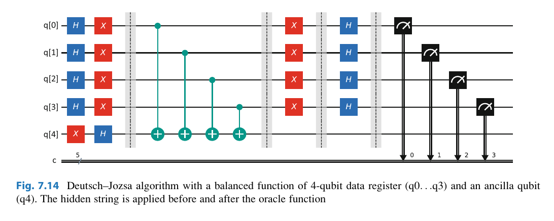
For the quantum version we have the following:

Pasted image 20240514135454.png

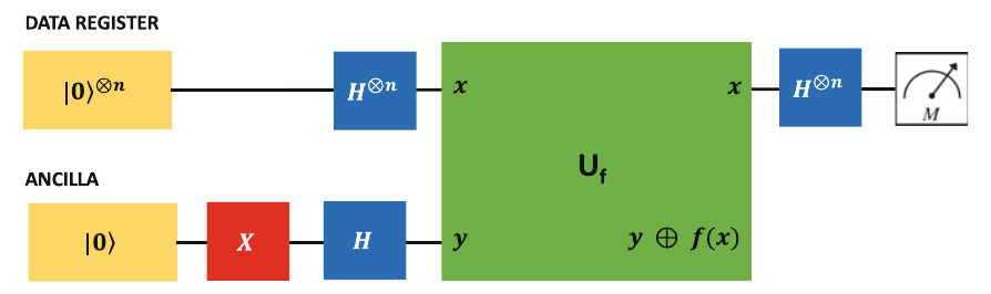
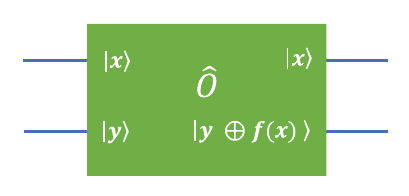
This ciruit uses an $n$ qubit data register and an ancilla qubit
The black box $U_{f}$ implements the oracle function $y \oplus f (x)$

We do the following:

Start the system with the data register and acnilla qubit initialized to $| 0 ⟩$ 's

| ψ ⟩ = {| 0 ⟩}^{\otimes n} | 0 ⟩

Apply an $X$ gate to the ancilla qubit to flip it to a $| 1 ⟩$ . We have $| ψ ⟩ = {| 0 ⟩}^{\otimes n} | 1 ⟩$
Apply $H$ to both the data register bits and the ancilla bits. For the data register, in general:

H^{\otimes n} | x_{1} . . . x_{n} ⟩ = ⨂_{i = 1}^{n} H | x_{i} ⟩

As such, for the $H$ gate in general:

H^{\otimes n} {| 0 ⟩}^{\otimes n} = \frac{1}{\sqrt{2^{n}}} \frac{1}{\sqrt{2^{n}}} (| 000. . .0 ⟩ + | 000. . .1 ⟩ + \dots + | 111. . .1 ⟩)

Which we can rewrite as:

H^{\otimes n} {| 0 ⟩}^{\otimes n} = \frac{1}{\sqrt{2^{n}}} \sum_{x = 0}^{2^{n} - 1} {| x ⟩}^{\otimes n} = \frac{1}{\sqrt{2^{n}}} \sum_{y = 0}^{2^{n} - 1} (- 1)^{x \cdot y} {| y ⟩}^{\otimes n}

where $x \cdot y$ is the bitwise inner product mod 2 as $x \cdot y = x_{0} y_{0} \oplus x_{1} y_{1} \oplus \dots \oplus x_{n - 1} y_{n - 1} \mod 2$ , allowing for operations like $H^{\otimes n}$ to happen on all $2^{n}$ possible states (allowing for exponential parallelism).

As such, for our steps above we have:

H^{\otimes n} {| 0 ⟩}^{\otimes n} = \frac{1}{\sqrt{2^{n}}} \sum_{x = 0}^{2^{n} - 1} | x ⟩

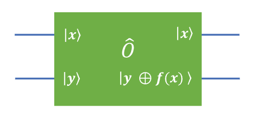
getting back to our circuit, apply $H$ gates to both the data register and ancilla bits (step 3):

H^{\otimes n} {| 0 ⟩}^{\otimes n} H | 1 ⟩ = \frac{1}{\sqrt{2^{n + 1}}} \sum_{x = 0}^{2^{n} - 1} | x ⟩ \underset{Applied from Second H}{\underset{⏟}{(| 0 ⟩ - | 1 ⟩)}}

By applying the oracle function $y \oplus f (x)$ into the ancilla qubit, we get:

\begin{aligned} y \oplus f (x) & = \frac{1}{\sqrt{2^{n + 1}}} \sum_{x = 0}^{2^{n} - 1} | x ⟩ ([| 0 ⟩ - | 1 ⟩] \oplus f (x)) \\ = \frac{1}{\sqrt{2^{n + 1}}} \sum_{x = 0}^{2^{n} - 1} | x ⟩ (| 0 \oplus f (x) ⟩ - | 1 \oplus f (x) ⟩) \\ = \frac{1}{\sqrt{2^{n + 1}}} \sum_{x = 0}^{2^{n} - 1} | x ⟩ (| f (x) ⟩ - | 1 \oplus f (x) ⟩) \end{aligned}

Focus on the term $| f (x) ⟩ - | 1 \oplus f (x) ⟩$ .

If $f (x) = 0$ then this term evaluates to $| 0 ⟩ - | 1 \oplus 0 ⟩ = | 0 ⟩ - | 1 ⟩$
If $f (x) = 1$ then this term evaluates to $| 1 ⟩ - | 1 \oplus 1 ⟩ = | 1 ⟩ - | 0 ⟩$

Thus we can write this term as $(- 1)^{f (x)} (| 0 ⟩ - | 1 ⟩)$ . Substituting:

y \oplus f (x) = \frac{1}{\sqrt{2^{n + 1}}} \sum_{x = 0}^{2^{n} - 1} | x ⟩ (- 1)^{f (x)} (| 0 ⟩ - | 1 ⟩)

Note

The ancilla qubit is unchanged from this operation!

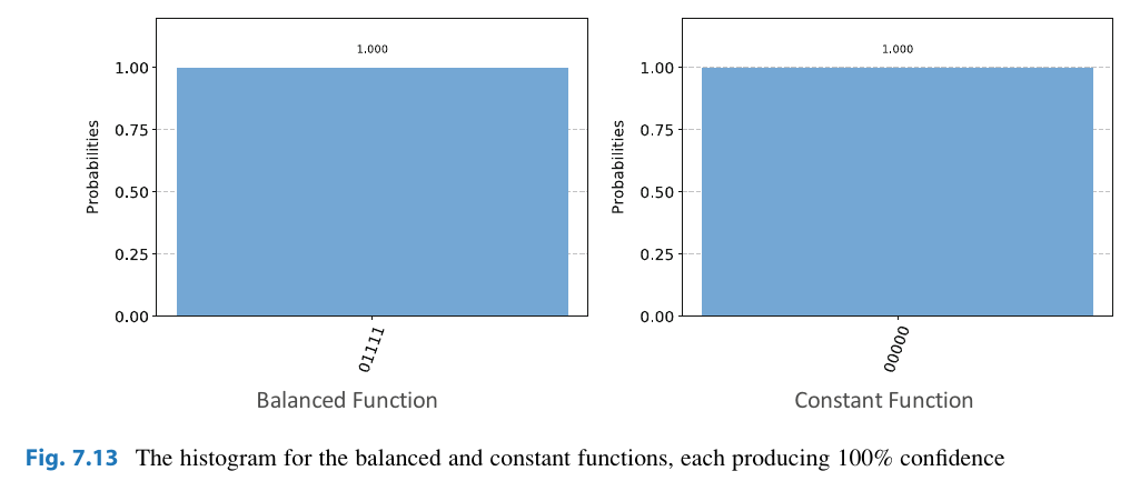
We don't need the ancilla qubit so we can drop it. The final step is to apply $H$ gates to the data register (step 4). Using the right side of this equation, we get:

\begin{aligned} y \oplus f (x) & = \frac{1}{\sqrt{2^{n}}} \sum_{x = 0}^{2^{n} - 1} (- 1)^{f (x)} H^{\otimes n} | x ⟩ \\ = \frac{1}{\sqrt{2^{n}}} \sum_{x = 0}^{2^{n} - 1} (- 1)^{f (x)} \cdot \frac{1}{\sqrt{2^{n}}} \sum_{y = 0}^{2^{n} - 1} (- 1)^{x \cdot y} | y ⟩ \\ = \sum_{y = 0}^{2^{n} - 1} (\frac{1}{2^{n}} \sum_{x = 0}^{2^{n} - 1} (- 1)^{f (x)} \cdot (- 1)^{x \cdot y}) | y ⟩ & (x \cdot y = ⨁_{i = 0}^{n - 1} x_{i} y_{i}) \end{aligned}

At this state we are ready to measure the data register. We just want to make sure (really we only care about) that the data in there projects to ${| 0 ⟩}^{n}$ , that is, when $| y ⟩ = {| 0 ⟩}^{n}$ . For this case $y = 0$ therefore $x \cdot y = 0$ , so the probability amplitude associated with this state is given by:

\frac{1}{2^{n}} \sum_{x = 0}^{2^{n} - 1} (- 1)^{f (x)}

Whose probability is:

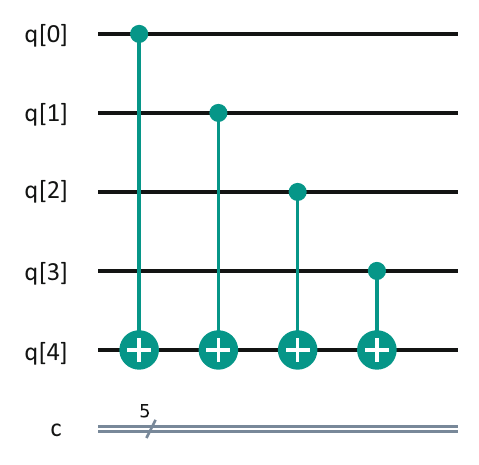
{| \frac{1}{2^{n}} \sum_{x = 0}^{2^{n} - 1} (- 1)^{f (x)} |}^{2} = {\begin{cases} 1 & for constant function \\ 0 & for balanced function \end{cases}

As a 4 qubit data register input:

Pasted image 20240515131822.png

The truth table for the balanced function would be:

Pasted image 20240515131837.png

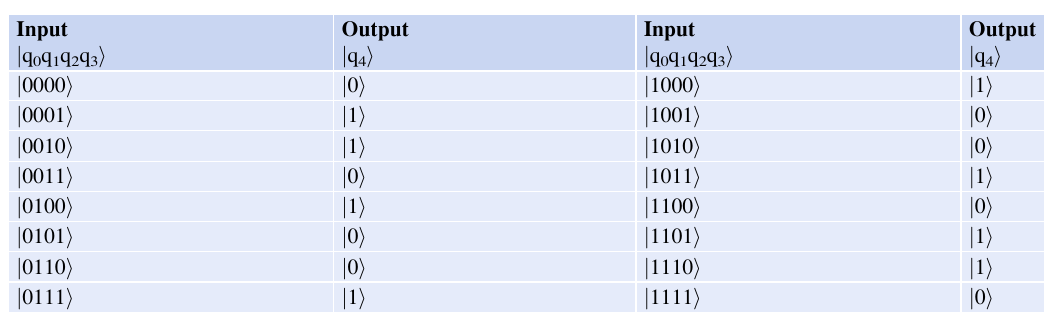
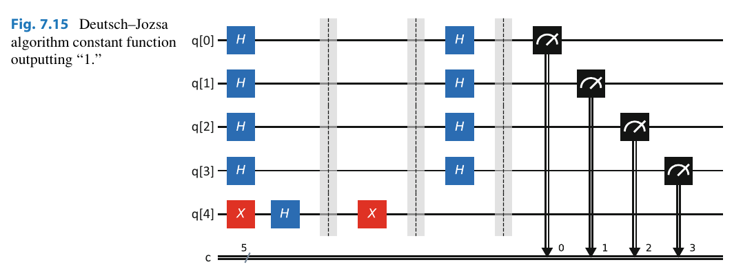
Notice here that the output $| q_{4} ⟩$ is counting the parity of the number of 1's in the input in this case. So if we have an odd number of $1$ 's we output a $| 1 ⟩$ and otherwise we output a $| 0 ⟩$ . Because there's an equal number of $| 0 ⟩$ 's and $| 1 ⟩$ 's then this function is balanced.

For a constant function, we can just:

If the ancilla qubit is $| 1 ⟩$ apply $X$ and get $| 0 ⟩$
If it's a $| 0 ⟩$ instead, don't do anything
This is a constant function of just $| 0 ⟩$ .

import qiskit
import math
from qiskit import *
from qiskit import IBMQ
from qiskit.visualization import plot_histogram, plot_gate_map
from qiskit.visualization import plot_circuit_layout
from qiskit.visualization import plot_bloch_multivector
from qiskit import QuantumRegister, ClassicalRegister, transpile
from qiskit import QuantumCircuit, execute, Aer
from qiskit.providers.ibmq import least_busy
from qiskit.tools.monitor import job_monitor
%matplotlib inline
%config InlineBackend.figure_format = 'svg'

# load the IBM Quantum account
account = IBMQ.load_account()

# Get the provider and the backend
provider = IBMQ.get_provider(group='open')
backend = Aer.get_backend('qasm_simulator')

# The balanced function
# qc – the quantum circuit
# n – number of bits to use
# input – the input bit string

def balanced_func (qc, n, input):
	# first apply the input as a bitmap to the data register
	for i in range (0, input.bit_length()):
		if ((1 << i) & input ):
			qc.x(i)
	qc.barrier()
	#setup the CNOT gates
	for i in range (n):
		qc.cx(i, n)
	qc.barrier()
	# apply the input one more time to restore state
	for i in range (0, input.bit_length()):
		if ((1 << i) & input ):
			qc.x(i)

# The constant function
# qc – the quantum circuit
# n – number of bits to use
# constant – set this to true for constant functions.
# False if not.
def constant_func (qc,n,constant=True):
	qc.barrier()
	# just apply a NOT gate to the ancilla qubit to output 1
	if (True == constant):
		qc.x(n)

# The Deutsch Jozsa algorithm
# qc – the quantum circuit
# n – the number of bits to use
# input – the input bit string
# function – set this to “constant” for constant functions.
# constant – set this to True for constant functions.
def deutsch_jozsa(qc, n, input, function, constant = True):
	# set the ancilla qubit to state 1.
	qc.x(n)
	#setup the H gates for both data register and ancilla qubit
	for i in range (n+1):
		qc.h(i)
	# call constant or balanced function as required
	if ("constant" == function ):
		constant_func(qc,n,constant)
	else:
		balanced_func(qc, n,input )
	qc.barrier()
	#setup the H gates for the data register and setup measurement
	for i in range (n):
		qc.h(i)
	qc.barrier()
	#measure the data register
	for i in range (n):
		qc.measure(i,i)

### MAIN CODE ###
number = 15 # The hidden string
numberofqubits = 5
shots = 1024

q = QuantumRegister(numberofqubits, 'q')
c = ClassicalRegister(numberofqubits, 'c')
qc = QuantumCircuit(q,c)

deutsch_jozsa(qc, numberofqubits - 1, number, "constant", True)
#qc.draw('mpl')

backend = Aer.get_backend("qasm_simulator")
job = execute(qc, backend=backend, shots=shots)
counts = job.result().get_counts()
plot_histogram(counts)

Pasted image 20240515133405.png

Pasted image 20240515133416.png

Pasted image 20240515133437.png

Steps of Deutsch-Josza Algorithm

Flip the ancilla bit to $| 1 ⟩$ using an $X$ gate.
Apply $H^{\otimes n}$ to all the data bits $| x ⟩$ , along with $H | y ⟩$ for our ancilla.
Apply our oracle function $y \oplus f (x) = \frac{1}{\sqrt{2^{n + 1}}} \sum_{x = 0}^{2^{n} - 1} | x ⟩ (| f (x) ⟩ - | 1 \oplus f (x) ⟩)$
Re-Hadamard our $| x ⟩$ bits. If we get a $1$ it is balanced. If we get a $0$ it is constant.

Ch 7.8: Grover's Search Algorithm

This algorithm uses amplitude amplification, a new technique that will be apparent in other algorithms. It specifically exhibits a quadratic speedup.

The algorithm is a search algorithm. Classical search algorithms would take $\frac{N}{2}$ attempts on average to find something (because we can't assume the thing we're searching is sorted so no binary search). Grover's algorithm solves this using an unstructured search because:

Our database isn't guarunteed to be sorted.
Takes a number corresponding to an entry in the database and performs a test to see if it's in there
Takes about $\frac{π}{4} \sqrt{N}$ steps so it's $O (\sqrt{n})$ .

Given a set of $N$ elements, namely $X = {x_{1}, . . ., x_{N}}$ and a given boolean function $f : X \to {0, 1}$ , the goal is to find an element $ω \in X$ such that $f (ω) = 1$ (ie: $ω$ has the desired condition we are looking for). Before starting, let's make the following assumptions:

The element $ω$ is unique, so only one $ω$ has it that $f (ω) = 1$
The size of the database is a power of 2, namely $N = 2^{n}$ . Padding can help us achieve this.
The data is labeled as $n$ -bit Boolean strings ${0, 1}^{n}$
The boolean function $f$ maps ${0, 1}^{n} \to {0, 1}$

Namely we can change $X = {000. . .001, 000. . .010, . . ., 111. . .111}$ so we have just a collection of binary numbers. While listed here in order and in completeness, the actual elements may be varied.

Let's assume we define an oracle function $\hat{O}$ which produces a transformation function:

O | x ⟩ \to | f (x) ⟩

Sadly this isn't unitary. It takes an $n$ -bit string and produces a single-bit output (so clearly $\hat{O}$ isn't invertible). Instead, use an oracle black-box function like we saw before w/ Deutsch-Jozsa:

Pasted image 20240522180748.png

As such, let's try to define our oracle function $\hat{O}$ acting on the $n$ -qubit input register $| x ⟩$ :

\hat{O} | x ⟩ = (- 1)^{f (x)} | x ⟩ = {\begin{cases} | x ⟩ & if f (x) = 0 \\ - | x ⟩ & if f (x) = 1 \end{cases}

Consider the block diagram below:

Pasted image 20240522181050.png

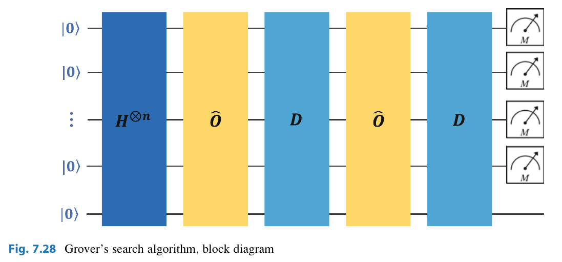
Here, we start with all the qubits at $| 0 ⟩$ . We apply a Hadamard transform to put the qubits in an equal superposition state:

| ψ ⟩ = \frac{1}{\sqrt{N}} \sum_{x \in {0, 1}^{n}} | x ⟩

All the qubits have the same amplitude $\frac{1}{\sqrt{N}}$ at this point. The next step is to apply the oracle $\hat{O}$ . The oracle function negates the amplitude of the state $ω$ . The rest of the states remain unaffected by the oracle:

| ψ ⟩ = \frac{- 1}{\sqrt{N}} | ω ⟩ + \frac{1}{\sqrt{N}} \sum_{x \in {0, 1}^{n}, x \neq ω} | x ⟩

Pasted image 20240522181749.png

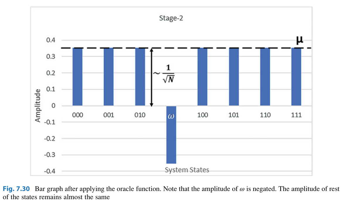
You can see this effect on the top bar graph.

Now that the amplitude of $| ω ⟩$ has changed, let's calculate the average of the amplitudes to ascertain we are on the right path. The average $μ$ is given by the following equation:

μ = \frac{1}{N} \sum_{x =\in {0, 1}^{n}} a_{x}

where here $a_{x}$ is the amplitude of a given $x \in {0, 1}^{n}$ . We can exapnd the equation to calculate the value of $μ$ at this point:

\begin{aligned} μ & = \frac{1}{N} \sum_{x \in {0, 1}^{n}} a_{x} \\ = \frac{1}{N} (\underset{x \neq ω}{\underset{⏟}{\frac{2^{n} - 1}{\sqrt{N}}}} - \underset{ω}{\underset{⏟}{\frac{1}{\sqrt{N}}}}) \\ = \frac{2^{n} - 2}{\sqrt{N}} \\ \approx \frac{N}{N \sqrt{N}} & N = 2^{n} - 1 \approx 2^{n} - 2 as n is large \\ = \frac{1}{\sqrt{N}} \end{aligned}

Hence, the amplitude for most terms is about $\frac{1}{\sqrt{N}}$ . We see that the amplitude hasn't really changed since the term $\frac{- 1}{\sqrt{N}}$ is relatively insignificant for large $n$ .

We can now move on to the next part. This part is called the Grover diffusion operator, or the amplitude purification. It does the following:

\sum_{x \in {0, 1}^{n}} a_{x} | x ⟩ \to \sum_{x \in {0, 1}^{n}} (2 μ - a_{x}) | x ⟩

In our example, all non $ω$ states stay at the $2 μ - \frac{1}{\sqrt{N}} = \frac{1}{\sqrt{N}}$ point, while now:

ω = 2 μ - (\frac{- 1}{\sqrt{N}}) = \frac{3}{\sqrt{N}}

Pasted image 20240522182619.png

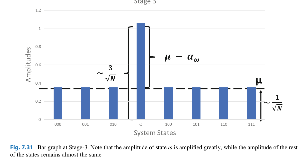
Both the steps of $\hat{O}$ and the oracle diffusion operator is called Grover Iteration. To amplify $ω$ more, just apply the iteration again. Let's do that:

Pasted image 20240522182705.png

We can see that for the $t$ -th iteration, then $ω$ gets amplified by $\sim \frac{t}{\sqrt{N}}$ (roughly). By applying this iteration $\sqrt{N}$ times, the amplitude of $ω$ should exceed $1$ , and at that point can reduce the overall $μ$ causing a reduction in the amplitude when the Grover Diffusion Operator is applied.

This is big! A classical implementation is $O (N)$ while this implementation is $O (\sqrt{N})$ ! The $\sqrt{}$ really comes from the fact that quantum parallelism computes $f (x)$ for all $N = 2^{n}$ states at the same time. In case there are multiple solutions $k$ to the problem, we would need $O (\sqrt{\frac{N}{k}})$ iterations.

Steps of the Grover Search Algorithm

Apply $H^{\otimes n}$ to get everything in a superposition
Apply our oracle $\hat{O} | x ⟩ = (- 1)^{f (x)} | x ⟩$
Apply Grover's Diffusion Operator: $\sum_{x \in {0, 1}^{n}} a_{x} | x ⟩ \to \sum_{x \in {0, 1}^{n}} (2 μ - a_{x}) | x ⟩$ where $μ$ is the average of the amplitudes $a_{x}$

3-qubit Implementation

We make an oracle encoding $ω = 010$ :

Pasted image 20240522183245.png

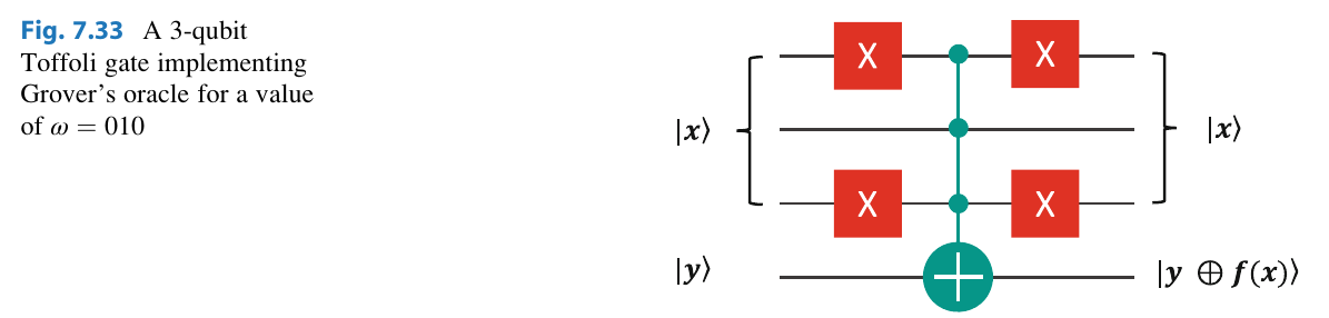
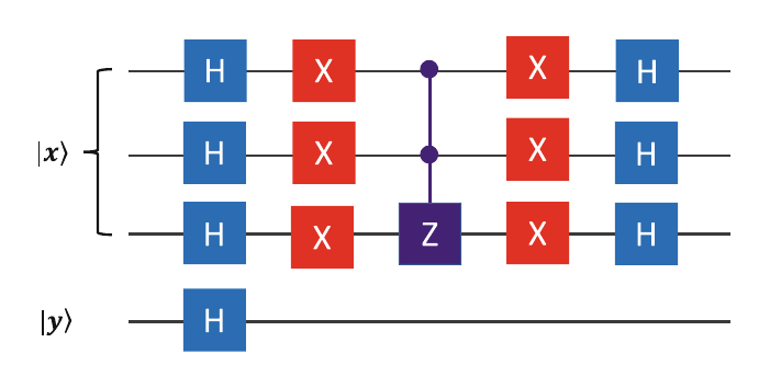
Then apply Grover's diffusion operator:

Pasted image 20240522183311.png

The goal of the oracle is to implement $\hat{O}$ that acts on $n$ -qubit input register $| x ⟩$ and the 1-qubit output register. The function applies $X$ to the output register when the input register is equal to $ω$ :

\hat{O} {| x ⟩}^{\otimes n} | y ⟩ = {| x ⟩}^{\otimes n} | y \oplus f (x) ⟩

Using the gate in Figure 7.33, we can implement $\hat{O}$ as a multi-control Toffoli (2-control NOT) gate. It switches the target $| y ⟩$ when all control registers are in $| 1 ⟩$

See the code listing below:

# The three control Toffoli gate
# qc - the quantum register
# control1, control2, control3 - The control registers
# anc - a temporary work register
# target - the target register, where the transform is applied

def cccx(qc,control1, control2, control3, anc, target):
	qc.ccx(control1,control2,anc)
	qc.ccx(control3,anc,target)
	qc.ccx(control1,control2,anc)
	qc.ccx(control3,anc,target)
	
# The Grover's Oracle
# qc - the quantum register
# x1, x2, x3 - The input register x
# anc - a temporary work register
# target - the target register, where the transform is applied

def grover_oracle( qc, x1, x2, x3, anc, target):
	qc.x(x3)
	qc.x(x1)
	cccx(qc, x1, x2, x3, anc, target)
	qc.x(x1)
	qc.x(x3)

# The CCZ gate
# qc - the quantum register
# control1, control2 - The control registers
# target - the target register, where the Z transform is applied
def ccz(qc, control1, control2, target):
	qc.h(target)
	qc.ccx(control1, control2, target)
	qc.h(target)
	
# The Grover's Diffusion Operator
# qc - the quantum register
# x1, x2, x3 - The input register x
# target - A temporary register
def grover_diffusion_operator(qc, x1, x2, x3, target):
	qc.h(x1)
	qc.h(x2)
	qc.h(x3)
	qc.h(target) # Bring this back to state 1 for next stages
	qc.x(x1)
	qc.x(x2)
	qc.x(x3)
	ccz(qc, x1, x2, x3 )
	qc.x(x1)
	qc.x(x2)
	qc.x(x3)
	qc.h(x1)
	qc.h(x2)
	qc.h(x3)

#
# Grover's algorithm
#
shots = 1024
q = QuantumRegister(3 , 'q')
t = QuantumRegister(2 , 't')
c = ClassicalRegister(3 , 'c')
qc = QuantumCircuit(q,t, c)

qc.h(q[0])
qc.h(q[1])
qc.h(q[2])
qc.h(t[0])

grover_oracle (qc, q[0], q[1], q[2], t[1], t[0])
grover_diffusion_operator (qc, q[0], q[1], q[2],t[0])

grover_oracle (qc, q[0], q[1], q[2], t[1], t[0])
grover_diffusion_operator (qc, q[0], q[1], q[2],t[0])

grover_oracle (qc, q[0], q[1], q[2], t[1], t[0])
grover_diffusion_operator (qc, q[0], q[1], q[2],t[0])

qc.measure(q[0],c[0])
qc.measure(q[1],c[1])
qc.measure(q[2],c[2])

backend = Aer.get_backend("qasm_simulator")
job = execute(qc, backend=backend, shots=shots)
counts = job.result().get_counts()
plot_histogram(counts)

To finish our discussion, let's derive the math. Start with the system ${| x ⟩}^{\otimes 3} | y ⟩$ in state $| 0 ⟩$ :

| ψ ⟩ = | 000 ⟩ | 0 ⟩

Then apply a NOT gate to $| y ⟩$ to get:

| ψ ⟩ = | 000 ⟩ | 1 ⟩

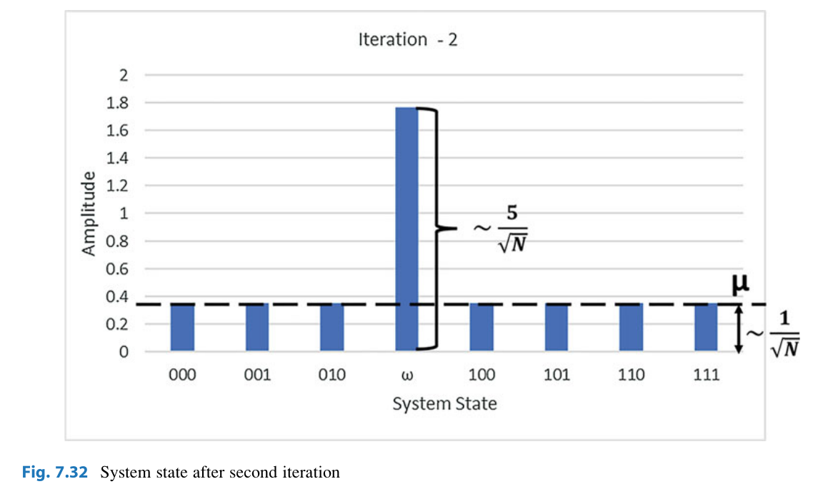
Then apply a $H$ to put the system in equal superposition state:

| ψ ⟩ = \frac{1}{\sqrt{8}} (| 000 ⟩ + | 001 ⟩ + | 010 ⟩ + | 011 ⟩ + \dots + | 111 ⟩) \otimes \frac{1}{\sqrt{2}} (| 0 ⟩ - | 1 ⟩)

Then apply Grover-Diffusion. The action of the $H$ gate on $| y ⟩$ changes it back to $| 1 ⟩$ . Since $μ = \frac{1}{\sqrt{8}}$ then the amplitudes of all state remain the same; however, the state of $ω$ becomes $3 / \sqrt{8}$ :

| ψ ⟩ = (\frac{1}{\sqrt{8}} (| 000 ⟩ + \dots + | 111 ⟩) + \frac{3}{\sqrt{8}} | 101 ⟩) \otimes | 1 ⟩

At the end of the second iteration, we now have a factor of $\frac{5}{\sqrt{8}}$ :

| ψ ⟩ = (\frac{1}{\sqrt{8}} (| 000 ⟩ + \dots + | 111 ⟩) + \frac{5}{\sqrt{8}} | 101 ⟩) \otimes | 1 ⟩

And after one last pass:

| ψ ⟩ = (\frac{1}{\sqrt{8}} (| 000 ⟩ + \dots + | 111 ⟩) + \frac{7}{\sqrt{8}} | 101 ⟩) \otimes | 1 ⟩