1.6: Wavefunctions and Probability Amplitudes

See Reading Week 1 - Quantum Cryptography, Computation, Teleportation; Review of Wave Functions and Young's Slit Experiment#1.6 Wavefunctions and Probability Amplitudes.

2.8: Eigenstates, Eigenvalues, and Eigenfunction

We learned that when linear operator $\hat{O}$ acts on a ket $|V⟩$, it transforms the ket into a new ket $|V^{\prime }⟩$. It's clert that, depending on the values of $\hat{O}$ that $|V^{\prime }⟩$ may be a different "shape", namely it may not be a scalar multiple of itself. There may be certain kets that when the action of $\hat{O}$ happens, it only gets scaled:

Such kets $|\psi ⟩$ are known as eigenkets, where $|\psi ⟩$ is an eigenket of the operator $\hat{O}$. The wavefunction $\psi$ is called an eigenstate. This is because the ket above $|\psi ⟩$ is independent of any observable. Projecting the ket into an observable basis (like position or momentum) then $\psi$ becomes a function of that observable. In these cases then $\psi$ is an eigenfunction. The value $a$ is the eigenvalue, and the equation above is called an eigenvalue equation. The set of eigenvalues is its spectrum. The eigenvectors corresponding to the distinct eigenvalues $a_1,...,a_n$ form a sub-space called the eigenspace.

If $\hat{O}$ is hermitian, then ${\mathrm{\Psi }}_a$ is the eigenstate and $a$ is the eigenvalue. Thus:

Similarly:

Thus the variance is:

Thus, we can deterministically measure quantity $O$ to the same value $a$, and the eigenstate ${\mathrm{\Psi }}_a$ is uniquely attached to the eigenvalue $a$ for the Hermitian operator $\hat{O}$.

If two eigenstates ${\mathrm{\Psi }}_a$ and ${\mathrm{\Phi }}_a$ of the same hermitian operator $\hat{O}$ correspond to the same eigenvalue $a$, then the states are said to be degenerate. Besides, the eigenstates ${\mathrm{\Psi }}_a$ and ${\mathrm{\Phi }}_a$ of a Hermitian operator, corresponding to difference eigenvalues $a_1$ and $a_2$ are othogonal.

Proof
In general mathematics, this comes from Lecture 10 - Adjoint in More Detail#^bfabbc, but specifically for quantum mechanics we can see that bra-ket notation here still works:

if we assume ${\mathrm{\Psi }}_i={\mathrm{\Psi }}_j=\mathrm{\Psi }$ and assume $\mathrm{\Psi }$ is normalized, then by using Reading Week 3 - Ending Quantum Superposition, Starting Qubits#^5cbb2b:

Which only happens unless $a$ is real.
☐
If we have ${\mathrm{\Psi }}_i\ne {\mathrm{\Psi }}_j$ then they have separate eigenvalues $a_i$ and $a_j$, so since $\hat{O}$ is Hermitian the eigenvalues are real. Besides, we can show that ${\mathrm{\Psi }}_i$ is orthogonal to ${\mathrm{\Psi }}_j$ if $a_i\ne a_j$ via:

so even if they are degenerate eigenfunctions, they are orthogonal.

The eigenfunctions form a complete set, where any function, even not itself an eigenfunction, can be written as a linear combintation of eigenfunctions:

this is the Quantum Superposition principle. Notice here that by the probability principle we require:

3.5: Postulates of Quantum Mechanics

We will list the important properties we can work with due to being in a Hilbert Space. There's a lot of mathematical properties we should know so that we can do the arithmetic at a higher level when possible.

3.5.1: Postulate 1

A QM system is given by some $\mathrm{\Psi }(\overrightarrow{r},t)$ which is complex. Here $\mathrm{\Psi }$ is:

• continuous
• square-integrable
• single-valued

The probabilistic interpretation of $\mathrm{\Psi }$ is ${\mathrm{\Psi }}^{\ast }\mathrm{\Psi }dV$, saying that the QM system is within volume element $dV$ at position $\overrightarrow{r}$ and at time $t$. $\mathrm{\Psi }$ is spatially localized (ie: normalized), and since it should be found anywhere in space, then ${\int }_{-\mathrm{\infty }}^{\mathrm{\infty }}{\mathrm{\Psi }}^{\ast }\mathrm{\Psi }dV=1$. The state-space of the wave function is the Hilbert Space, so the superposition principle holds good.

3.5.2: Postulate 2

Every observable in QM corresponds to a linear Hermitian operator:

• The expectation value of an operator corresponding to an observable is a real value. So the operator must be Hermitian via Reading Week 3 - Ending Quantum Superposition, Starting Qubits#^e5ce77. Hence, the measured quantities are real values.
• Every operator has got some states which do not change when the operator operates on them, namely $\hat{A}|\mathrm{\Psi }⟩=a|\mathrm{\Psi }⟩$. The states are just multiplied by a constant, and are called eigenstates. The constants $a$ are the eigenvalues of the operator $\hat{A}$.

3.5.3: Postulate 3

A QM measurement is observable, where the only possible outcome is one of the eigenvalues of the corresponding operator. We can write the system state as a linear combination of probability amplitudes:

Here $n\to \mathrm{\infty }$ is allowed. Here we have $\hat{A}|{\mathrm{\Psi }}_i⟩=a_i|{\mathrm{\Psi }}_i⟩$. Even though we may have infinitely many $a_i$'s, the measurement operation produces only one $a_i$ with a probability of 1, where the probability of which eigenvalue we measure is $|c_i{|}^2$. When we measure $|\mathrm{\Psi }⟩$ we get an $a_i$ for a certain $i$. This causes the wavefunction to collapse to $|{\mathrm{\Psi }}_i⟩$ and $|c_i{|}^2=1$. If $a_i$ is degenerate via Reading Week 3 - Ending Quantum Superposition, Starting Qubits#2.8 Eigenstates, Eigenvalues, and Eigenfunction then the wavefunction collapses to one of the degenerate subspaces.

The probability of measuring a certain eigenvalue $a_i$ is given by:

where $|{\mathrm{\Psi }}_i⟩$ is an eigenket of $A$, corresponding to eigenvalue $a_i$ to which the system collapses after the measurement.

3.5.4: Postulate 4

The average value or the expectation value of an observable is defined as:

The expectation value is the average of all measurements made on quantum systems prepared with the same state.

3.5.5: Postulate 5

The wavefunction of an isolated quantum system evolves in time following the time-dependent Shrodinger equation:

where $\hat{H}$ is the Hamiltonian operator of the system. Once given an initial state $\mathrm{\Psi }(\overrightarrow{r},t_o)$ it is possible to derive the state of the system, which cannot be determined by the time-dependent Schrodinger equation. When we measure a physical quantity of the system, the state vector undergoes a probabilistic change, which can be observed in the measurement outcome.

3.5.6: Symmetric and Antisymmetric Wavefunctions

Consider a system of two identical particles. Sine the particles are indistinguishable, under the exchange of coordinates (which includes spin), the probability density should not be affected. For such systems, the probability density of the wavefunctions describing the two particles must be identical:

this happens when (either or):

1. The wavefunction is symmetric, so $\mathrm{\Psi }(r_1,r_2)=\mathrm{\Psi }(r_2,r_1)$
2. The wavefunction is antisymmetric, so $\mathrm{\Psi }(r_1,r_2)=-\mathrm{\Psi }(r_2,r_1)$.
   This gives rise to the Pauli-Exclusion Principle, derived from antisymmetric wavefunctions.

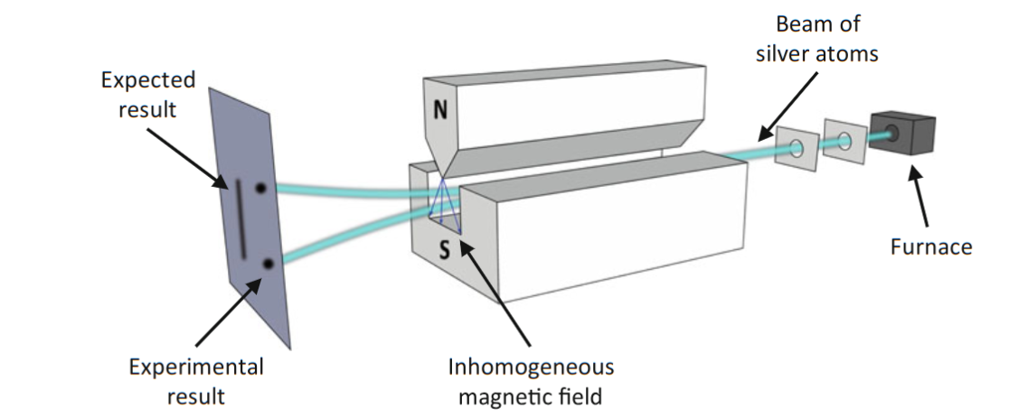
3.7: Stern and Gerlach Experiment

Recall from Chapter 1 that the orbital angular momentum quantum number $l$ only takes discrete integer values. Thus, the angular momentum vector can only have certain orientations called space quantization.

The beam of neutral silver atoms passes through an inhomogeneous magnetic field and hits a target screen. If the direction of bean is the $y$-axis and the magnetic field along the $z$-axis, then the electrons in a circular orbit have an angular momentum $\overrightarrow{L}=m\omega r^2$. Since the electrons in orbit carry a charge, they produce a small current loop around them, creating a dipolar magnetic field and a magnetic moment $\mu =-\frac{2}{2m}\overrightarrow{L}$.

The magnetic field $\overrightarrow{B}$ created by the experiment creates a torque $\mu \times \overrightarrow{B}$ around this dipole such that $\overrightarrow{L}$ starts to precess along the direction of the magnetic field:

the random thermal effects of the furnace should deflect the particles as various $\pm z$ values, thus expecting the continuous line shown above. What really happened were the dots, so the force that deflects the beam must have discrete values, hence spatial quantization.

The silver atoms are actually in a $L=0$ state, and if $L=1$ instead then the magnetic quantum number $m$ must have $2L+1=3$ states, expecting 3 dots. But they actually still only got 2.

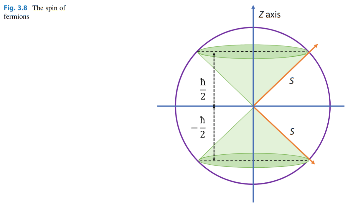
Uhlenbeck, Goudsmit proposed the theory that in addition to the orbital angular momentum $L$, the electrons have an intrinsic angular momentum or the spin angular momentum $S$ with the value $\frac{\hslash }{2\pi }$:

The total angular momentum is the sum of the orbital and spin angular momentums:

Silver has electron configuration $4d^{10}5s^1$ so the one valence electron in $n=5$, while the remaining electrons have a total angular momentum of 0 (the spins cancel out). The electron doesn't have orbital angular momentum ($L=0$), but rather just the spin angular momentum. The experimental observation is from this spin alone! The spin can have two different values, and electrons are spin-1/2 particles. The same is true for other fermions.

If we measure the spin along the direction of the $z$-axis, the two spin states are:

similar with the other axes:

We say $S_z=+1/2\hslash$ is the spin upward $\uparrow$ state and $S_z=-1/2\hslash$ is the downward $\downarrow$ state. We can say:

We can define a spin operator $\widehat{S_z}$ with the two eigenstates having eigenvalues $\pm 1/2\hslash$. Thus:

We can just relabel $\uparrow$ as $0$ and $\downarrow$ as $1$, with the corresponding standard basis as well:

The bra-versions can be gotten by taking the conjugate transpose. Thus:

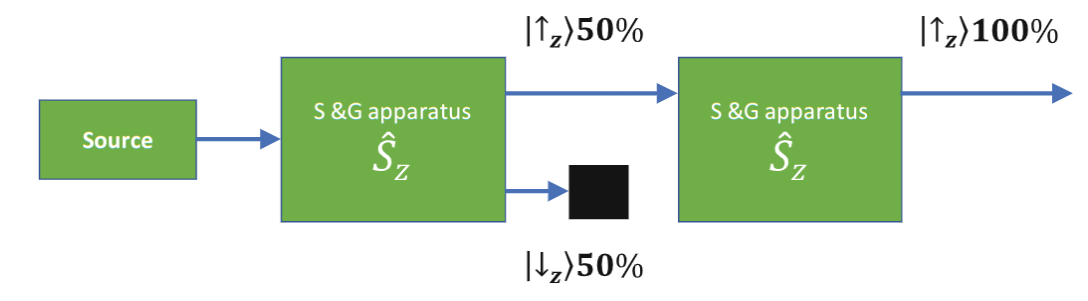
if we cascade two Stern/Gerlach apparatuses, where the first randomly gives 50% precedence to each up/down state. We feed the ${\uparrow }_z$ output to the second apparatus, leaving our ${\downarrow }_z$. This let's all the ${\uparrow }_z$ pass with 100% probability to the next apparatus:

Thus, then each vector combination $⟨i|j⟩=\chi (i=j)$. So:

so then put these in the matrix:

Start of Lecture Slides: Quantum Superposition

![[Physics CPE 345 Quantum Computing Lecture slides Week 2 Quantum superposition 240415 2 for web.pdf#page=1]]

3.8: Bloch Sphere Representation

In Reading Week 3 - Ending Quantum Superposition, Starting Qubits#3.7 Stern and Gerlach Experiment we talked about the $\uparrow$ and $\downarrow$ states, and that these spins are always $\hslash /2$. These states are referred to a qubit meaning quantum bits.

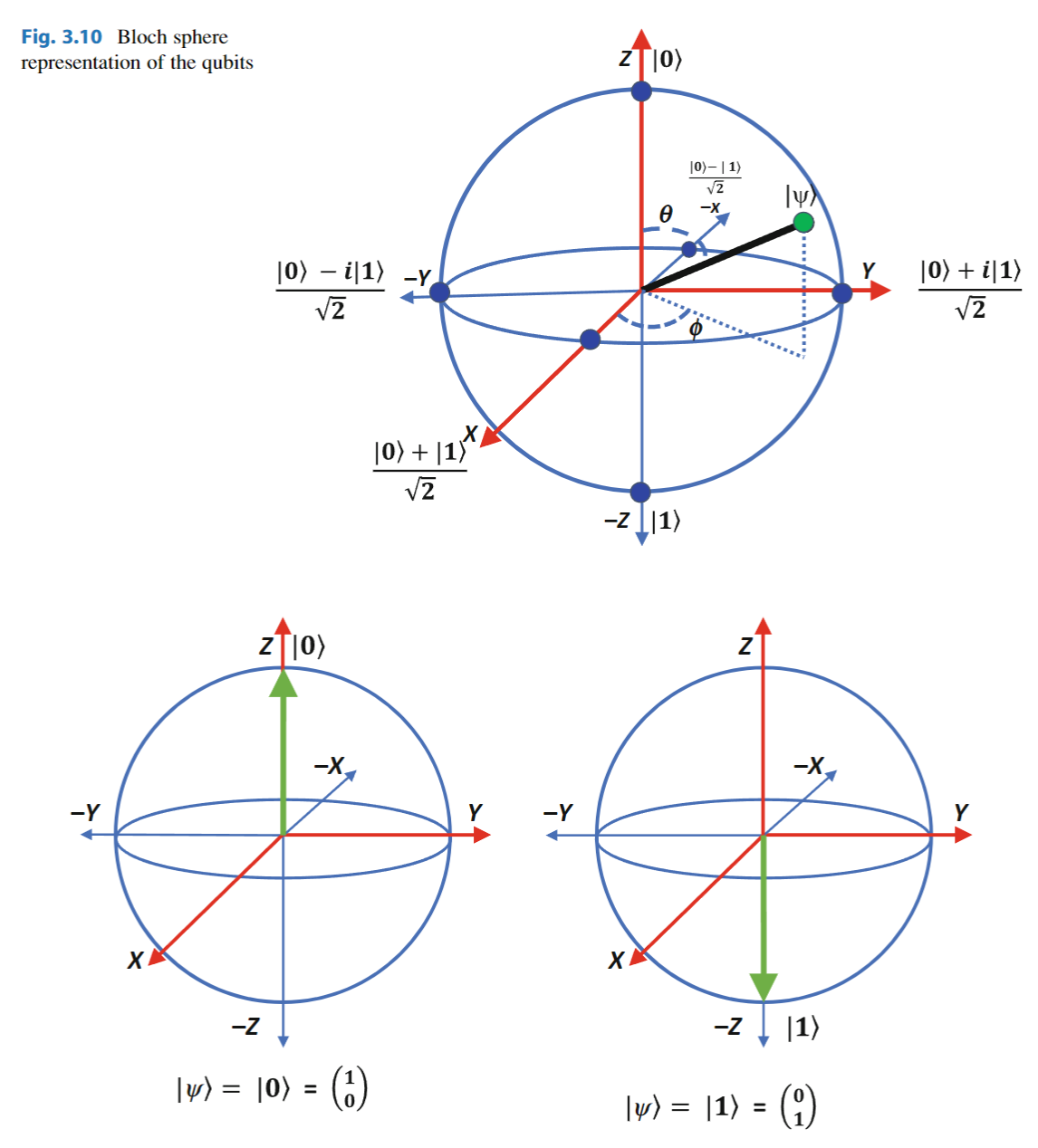
Recall that any wavefunction $\psi$ is a superposition of these states, which we relabel with $|0⟩$ and $|1⟩$ respectively:

where using $|\uparrow ⟩$ and $|\downarrow ⟩$ refers to the standard basis, while using $|0⟩$ and $|1⟩$ refers to the computational basis. The relative phase between $a$ and $b$ is responsible for quantum interference.

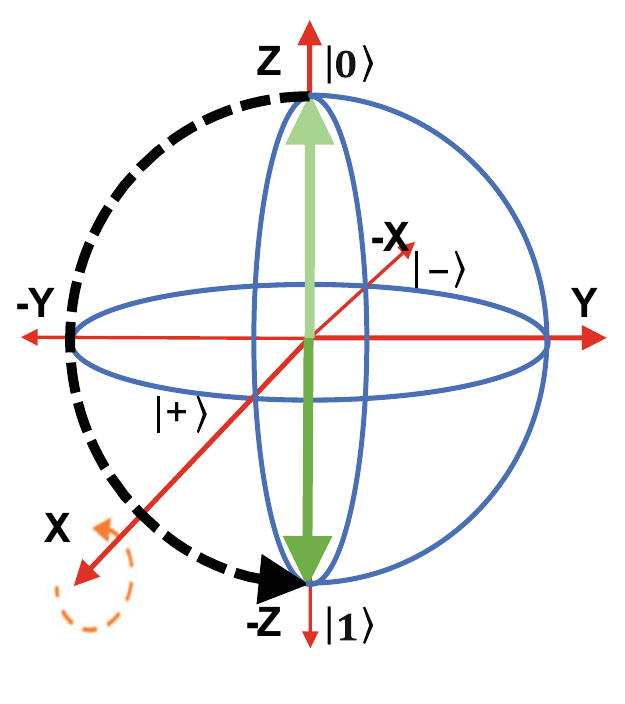
The state vector can be drawn as a vector pointing to the surface of a unit sphere called the Bloch Sphere:

Using a spherical coordinate system, an arbitrary position of the state vector of a qubit can be written in terms of the angle $\theta$ (elevation) and $\varphi$ (azimuth, the angle of projection into the $xy$-plane):

We can measure the direction of the qubit's state vector by directing a magnetic field $\overrightarrow{B}$ along the $z$-axis and measuring the energy. This will be the same direction as the expectation value vector of $\widehat{S_z}$.

Here, the probability is given by the $|a_i{|}^2$ terms for each state $|i⟩$. If we have $|\psi ⟩=(a,b{)}^{\ast }$ then:

3.8.1: Qubit Rotations

The Pauli matrices rotate the state vector 180 degrees along their respective axes. These operations are called gates.

3.8.1.1 Pauli $X$-Gate

This rotates a qubit 180 degrees along the $x$-axis:

3.8.1.2 Pauli $Y$-Gate

This rotates a qubit 180 degrees along the $y$-axis:

3.8.1.3 Pauli $Z$-Gate

This rotates the qubit by 180 along the $z$ axis:

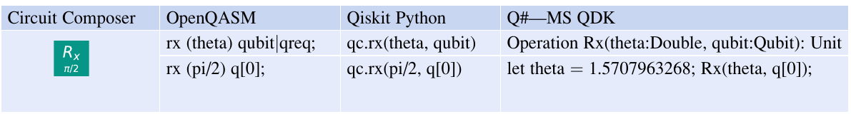
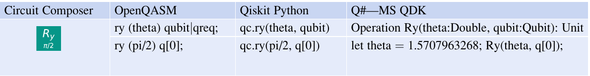
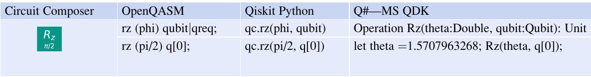
3.8.1.4: Rotation Operator

The general form of the rotation operator $\hat{R}$ is given by the equation:

where $\hat{n}$ is the unit vector along the axis of rotation, $\theta$ is the angle to be rotated, and $\sigma$ is the corresponding Pauli matrix. For example, to rotate around the $y$-axis we do:

similarly:

here we Pauli matrices ${\sigma }_i$ are equal to these matrices at 180 degrees:

and so on for ${\sigma }_y,{\sigma }_z$.

3.9: Projective Measurements

Sometimes, we need to make a measurement of a system via a change of basis, via new vector $|0^{\prime }⟩,|1^{\prime }⟩,...$ and so on. There's actually a really cool way to make the method to measure these, and its the projection operators.

In QM, projective measurement is described by observable $M$, and operator defined in the same $\mathbb{H}$. If the eigenvalues $m$ are the possible outcomes of the measurement, then we write $M$ as:

where $P_m$ are the complete set of orthogonal projectors onto the eigenspace of $M$. If we assume a state of the system before the measurement is $|\psi ⟩$ then the following axioms hold:

1. The total probability of all measurements is 1: $\sum _m{P}_m=I$ where $I$ is the identity matrix.
2. The probability of getting a certain measurement $m$ is $p(m)=⟨\psi |P_m|\psi ⟩$. This comes from how if we project $|\psi ⟩$ onto any $|i⟩$ basis vector then we get:

Thus, then $p(i)=|⟨i|\psi ⟩{|}^2=⟨\psi |P_i|\psi ⟩$.
3. The state of a system after the measurement is:

Measurements collapse the system into one of the states. This abrupt change is the projection postulate. The outcome of the measurement is a new state, which is the normalized projection of the original system ket into the ket corresponding to the measurement.

Here the operators of the projective measurements are called projectors, where $P^2=P$, so you only need to apply them up to one time. Here any $P_i$ where $i$ is the $i$-th basis vector is:

The probability of measuring the system in state $|i⟩$ is done via:

as expected. Note that that is how we derive:

The average value of the measurement then will be:

We can then define the standard deviation as:

3.9.2: Measuring Multi-Qubit Systems

Consider our standard 2 states. Notice if $|{\psi }_1⟩=a_1|0⟩+b_1|1⟩$ and $|{\psi }_2⟩=a_2|0⟩+b_2|1⟩$ then:

We can then just define a new set of states as shown above. Here, still:

In most cases, we can just measure one of the qubits (see entanglement later on). If we measure the first qubit along, we can distinguish between $00$ and $01$, so the operator that measures the first qubit in state $|0⟩$ must have projectors for the states $00$ and $01$:

... (a lot of info on projectors is irrelevant and just cool to know)

3.9.3: Measurements

Similar to using a voltmeter to measure voltage, to measure observable $Q$ of a quantum system $S$ we bring it in proximity with a meter $M$ and allow them to act linearly.

Suppose $|\psi ⟩=\sum a_i|x_i⟩$ and the meter is in state $|m⟩$. The composite of the state of the system $S+M$ is given by:

Here $|x_i⟩$ are the eigenvectors of $Q$ and the possible outcomes of the measurements are $q_i$. Measuring the measurements $q_i$ gives the state in the system:

where $m_i$ are orthonormal vectors, namely $a|0⟩|m_0⟩+b|1⟩|m_1⟩$. Due to the measuremnt process, the system "collapses" from the $\sum {\gamma }_i...$ state to the $|x_i⟩\otimes |m_i⟩$ for some $i$.

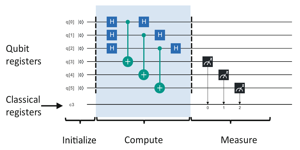
5.3: Introducing Quantum Circuits

Similar to classical computers, we construct a quantum circuit to implement a quantum algorithm. Each circuit solves a specific problem using unitary operations in the Hilbert space, assuming finite numbers of qubits.

Since there's unitary operations, the quantum circuits have the same number of inputs as outputs. Further, the quantum circuits are acyclic, lacking any feedback loops.

Every quantum circuit is just a set of matrix operations using unitary matrices, thus $U_{qc}$ that represents our quantum circuit has some inverse $U_{qc}^{-1}=U_{qc}^{\ast }$ by the definition of unitary, so all quantum circuits are reversible. If we start from the output, we should be able to retrieve the inputs, so information is preserved.

There's three stages to a QC:

1. Initialize: prepare a certain number of qubits
2. Compute: do our gate operations
3. Measure: measure the states of the qubits via projection to classical bits

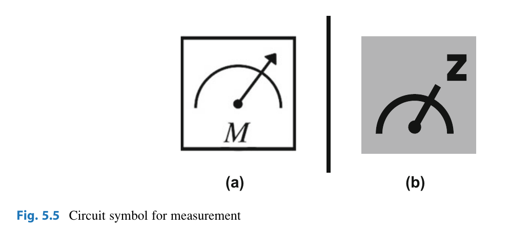
5.3.1: On Quantum Measurements

We describe the quantum state of a qubit via:

When measuring, we project to the states $|0⟩$ or $|1⟩$, where the probability of which we measure is determined by $a,b$.

Note:

• Some places use $M$ to denote the measurement
• Others denote $Z$ since we usually are measuring particle spin on the $z$-axis.

Keep in mind when measuring that the probability for getting $|0⟩$ is $|a{|}^2$ and for $|1⟩$ is $|b{|}^2$. As such, most quantum systems will repeatedly measure the output to see what the approximate probability is.

5.4: Quantum Gates

If we start with a qubit in state $|\psi ⟩$ and apply unitary operation $U$, then the final state $|{\psi }^{\prime }⟩$ is given via:

here $U$ will be a $2^n\times 2^n$ matrix, where $n$ is the number of qubits we have in our system.

5.4.1: Clifford Group Gates for Single Qubits

We have a list of gates to get through. Use this more as a good quick-reference where need be:

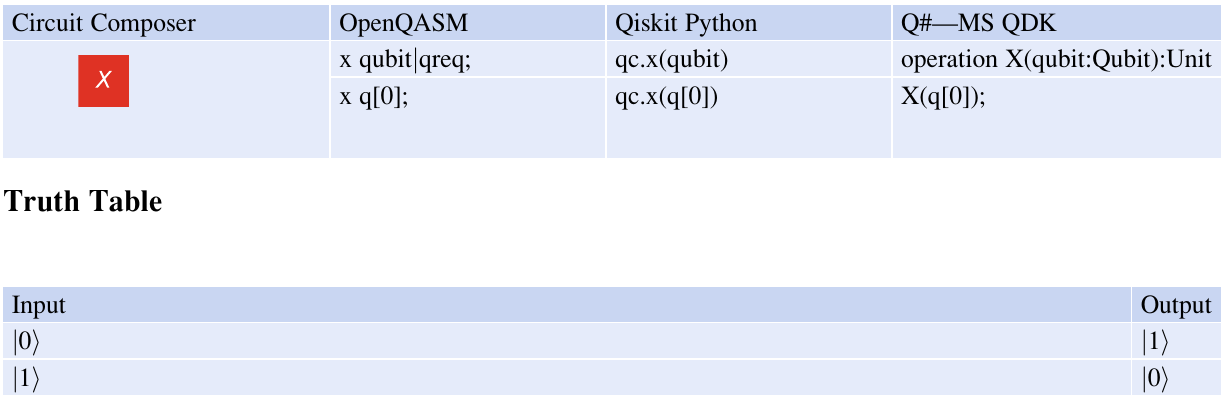
5.4.1.1: The Bit-Flip Gate, NOT Gate, Pauli-$X$ Gate

This gate applies a $\pi /2$ rotational pulse around the $x$-axis, flipping the state from $|0⟩$ to $|1⟩$ and vice versa

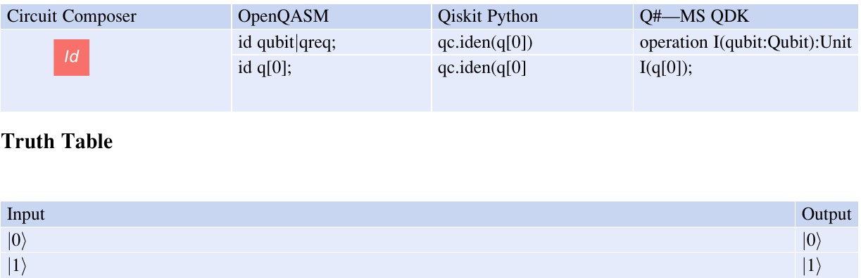
5.4.1.2: The Identity Gate

The gate does nothing:

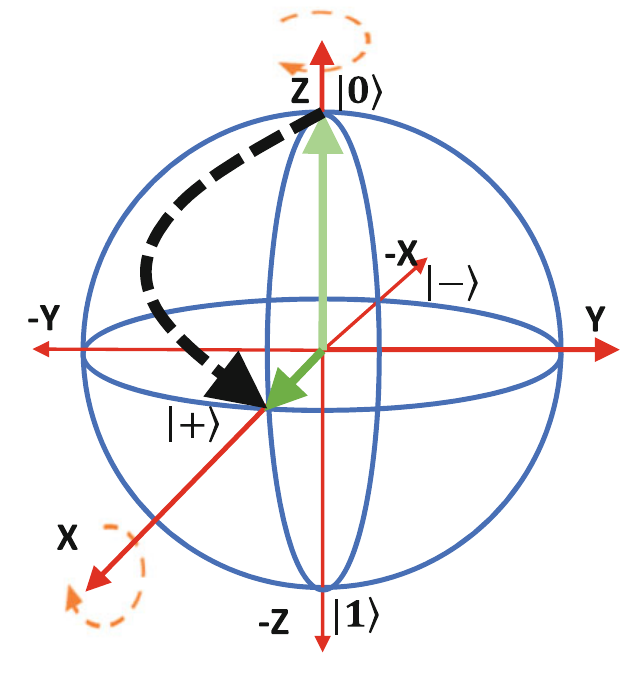
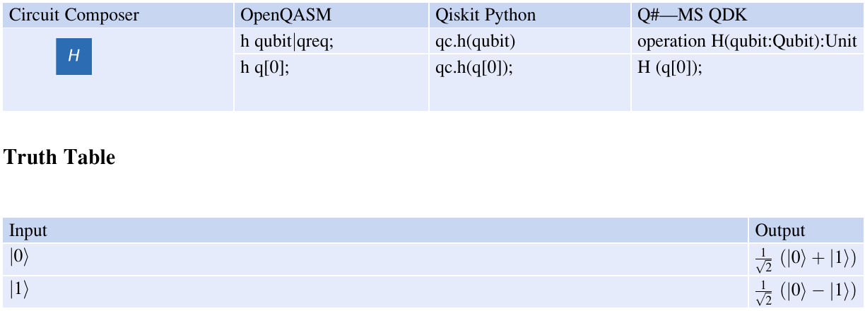
5.4.1.3: The Hadamard Gate, $H$-Gate

Rotates the qubit by $\pi$ radians along an axis diagonal to the $xy$-plane, equal to rotating the qubit by $\pi /2$ radians along the $y$-axis and then by $\pi /2$ degrees along the $x$-axis.

Here the $|+⟩,|-⟩$ are called the polar basis. Alternatively, we can write $H$ as:

Later on you may see this notation become:

because when we have multiple qubits, the summation will have to go across all of these possible states.

Alternative notation:

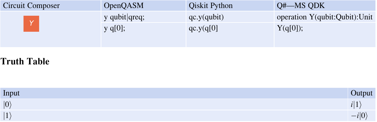
5.4.1.4: Pauli $Y$ Gate

Rotates the qubit along the $y$-axis by $\pi$ radians:

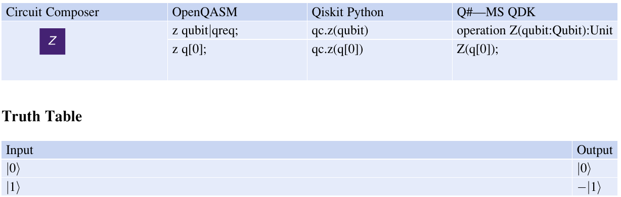
5.4.1.5: Pauli $Z$ Gate (Phase-flip Gate)

Rotate the qubit by $\pi$ radians along the $z$ axis:

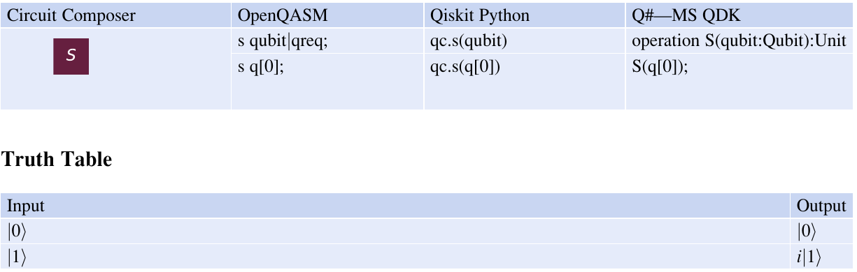
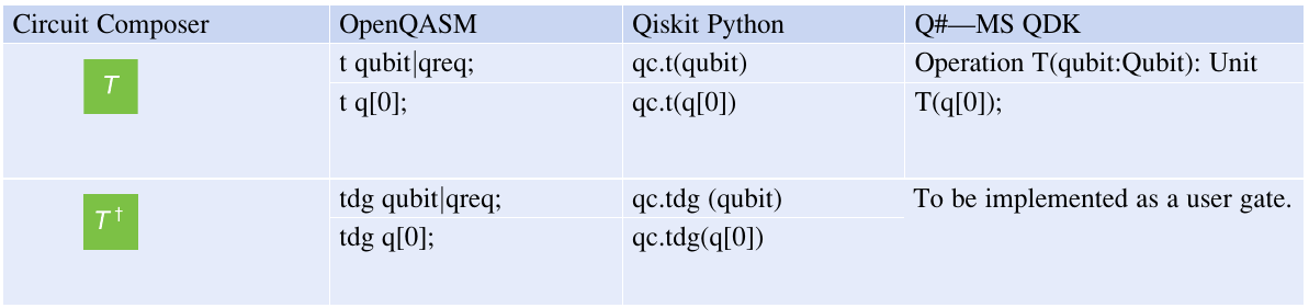
5.4.1.6: The $S$ Gate or $Z90$ Gate or Phase Gate

Rotates the qubit by $\pi /2$ radians along the $z$-axis. Some may refer to this gate as a $\pi /4$ phase gate:

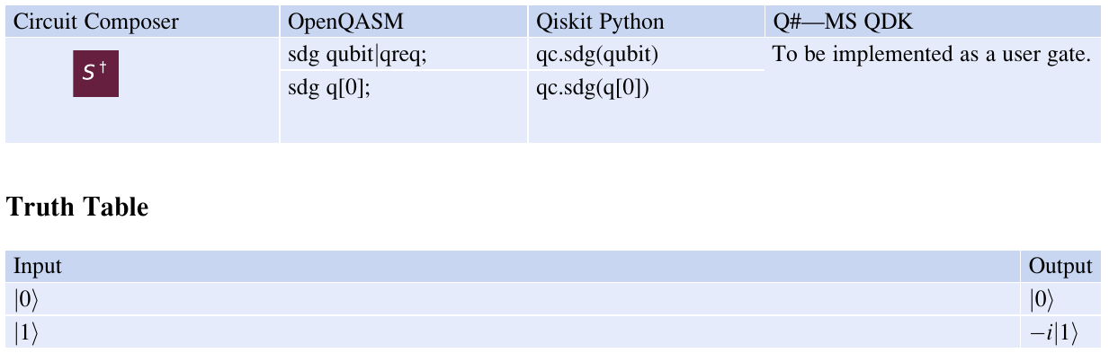
5.4.1.7: The $S^{\ast }$ Gate or the Sdag Gate

The $S^{†}$ gate is the conjugate transpose of the $S$ gate (and thus its inverse):

5.4.2: Arbitrary Rotation of the Qubit

We can rotate the qubits arbitrarily along the $x,y,z$ axes. In this section, we talk about the $R$ gates that can do it over any axes.

5.4.2.1: $RX$-Gate

Rotates the qubit along the $x$-axis by $\theta$ radians:

We can write these in terms of the Pauli Matrix $X$:

5.4.2.2: $RY$-Gate

Rotates the qubit along the $y$-axis by $\theta$ radians:

5.4.2.3: $RZ$-Gate

Rotates the qubit along the $z$ axis by $\varphi$ radians:

5.4.2.4: $T$ Gate and the $T^{†}$ Gate or the $\sqrt{S}$ Gate

These are cases of the $R_z$ gate with $\theta =\pm \frac{\pi }{4}$ and thus are the square root of $S$ (meaning $S^2$ is equivalent to these gates).

5.4.3: Physical Gates ($U$ Gates)

The $U$ gates you see mentioned above are implementable, and we talk about them here.

5.4.3.1: $U3$ Gate

Here $\theta ,\varphi$ are rotational angles in the bloch sphere and $e^{i\lambda }$ is a global phase.

and can similarly be found for the other $U$ gates.

5.4.3.2: $U2$ Gate

U_1(\lambda) = U_3(0,0,\lambda) = \begin{bmatrix}
1 & 0 \
0 & e^{i\lambda}
\end

U_1(\lambda)\ket{x} = e^{i\lambda x}\ket